ニューラルネットの学習過程の可視化を題材に、Jupyter + Bokeh で動的な描画を行う方法の紹介 [Jupyter Advent Calendar 2017]
Line https://bokeh.pydata.org/en/latest/docs/reference/models/glyphs/line.html

VBar https://bokeh.pydata.org/en/latest/docs/reference/models/glyphs/vbar.html

HBar https://bokeh.pydata.org/en/latest/docs/reference/models/glyphs/hbar.html

ImageRGBA https://bokeh.pydata.org/en/latest/docs/reference/models/glyphs/image_rgba.html
ImageRGBA https://bokeh.pydata.org/en/latest/docs/reference/models/glyphs/image_rgba.html

前置き
Jupyter Advent Calendar 2017 14日目の記事です。この記事は、Jupyter notebookで作成したものをnbconvertでmarkdownに変換し、手で少し修正して作りました。読み物としてはこの記事を、実行するにはノートブックの方を参照していただくのが良いかと思います。
概要
適当なニューラルネットの学習過程の可視化(ロス、正解率の遷移等)を題材にして、Bokehを使って動的にグラフを更新していくことによる可視化の実用例を紹介します。このノートブックの冒頭に、最後まで実行すると得られるグラフ一覧をまとめました。どうやってグラフを作るのか知りたい方は続きを読んでもらえればと思います。Bokehの詳細な使い方は、公式ドキュメントを参考にしてください。
なお、ここで紹介する例は、僕が過去に出た機械学習のコンペ (https://deepanalytics.jp/compe/36?tab=compedetail) で実際に使用したコードからほぼ取ってきました(8/218位でした)。グラフを動的に更新する方法は 公式ドキュメント に記述されていますが、そのサンプルの内容は「円を描画して色を変える」といった実用性皆無のものであること、またググっても例が多く見つからないことから、このような紹介記事を書くことにしました。参考になれば幸いです。
余談ではありますが、こと機械学習に関しては、tensorboardを使ったほうが簡単で良いと思います。僕は最近そうしています。 https://qiita.com/r9y9/items/d54162d37ec4f110f4b4. 色なり位置なり大きさなりを柔軟にカスタマイズしたい、あるいはノートブックで処理を完結させたい、と言った場合には、ここで紹介する方法も良いかもしれません。
%pylab inline
Populating the interactive namespace from numpy and matplotlib
from IPython.display import HTML, Image
import IPython
from os.path import exists

def summary():
    baseurl = "https://bokeh.pydata.org/en/latest/docs/reference/models/glyphs/"
    for (name, figname, url) in [
        ("Line", "line", "line.html"),
        ("VBar", "vbar", "vbar.html"),
        ("HBar", "hbar", "hbar.html"),
        ("ImageRGBA", "gray_image", "image_rgba.html"),
        ("ImageRGBA", "inferno_image", "image_rgba.html"),
        ]:
        gif = "./fig/{}.gif".format(figname)
        print("\n",name, baseurl + url)
        if exists(gif):
            with open(gif, 'rb') as f:
                IPython.display.display(Image(data=f.read()), format="gif")

summary()
(※ブログ先頭に貼ったので省略します)
# True にしてノートブックを実行すると、上記gifの元となる画像を保存し、最後にgifを生成する
save_img = False
if save_img:
    import os
    from os.path import exists
    if not exists("./fig"):
        os.makedirs("./fig")
    toolbar_location = None
else:
    toolbar_location = "above"

# bokehで描画したグラフはnotebookに残らないので、Trueの場合は代わりに事前に保存してあるgifを描画する
# もしローカルで実行するときは、Falseにしてください
show_static = True
準備
先述の通り、ニューラルネットの学習過程の可視化を題材として、Jupyter上でのBokehの使い方を紹介していきたいと思います。今回は、PyTorch (v0.3.0) を使ってニューラルネットの学習のコードを書きました。
https://github.com/pytorch/examples/tree/master/mnist をベースに、可視化しやすいように少しいじりました。
import torch
import torch.nn as nn
import torch.nn.functional as F
import torch.optim as optim
from torchvision import datasets, transforms
from torch.autograd import Variable
import numpy as np
Data
use_cuda = torch.cuda.is_available()

batch_size = 128

kwargs = {'num_workers': 1, 'pin_memory': True} if use_cuda else {}
train_loader = torch.utils.data.DataLoader(
    datasets.MNIST('./data', train=True, download=True,
                   transform=transforms.Compose([
                       transforms.ToTensor()
                   ])),
    batch_size=batch_size, shuffle=True, **kwargs)
test_loader = torch.utils.data.DataLoader(
    datasets.MNIST('./data', train=False, transform=transforms.Compose([
                       transforms.ToTensor(),
                   ])),
    batch_size=batch_size, shuffle=False, **kwargs)

data_loaders = {"train": train_loader, "test":test_loader}
Model
簡単な畳み込みニューラルネットです。
class Net(nn.Module):
    def __init__(self):
        super(Net, self).__init__()
        self.conv1 = nn.Conv2d(1, 10, kernel_size=5)
        self.conv2 = nn.Conv2d(10, 20, kernel_size=5)
        self.conv2_drop = nn.Dropout2d()
        self.fc1 = nn.Linear(320, 50)
        self.fc2 = nn.Linear(50, 10)

    def forward(self, x):
        x = F.relu(F.max_pool2d(self.conv1(x), 2))
        x = F.relu(F.max_pool2d(self.conv2_drop(self.conv2(x)), 2))
        x = x.view(-1, 320)
        x = F.relu(self.fc1(x))
        x = F.dropout(x, training=self.training)
        x = self.fc2(x)
        return F.log_softmax(x, dim=-1)
Train loop
from tqdm import tnrange
epochs = 20

def __train_loop(model, data_loaders, optimizer, epoch, phase):
    model = model.train() if phase == "train" else model.eval()
    running_loss = 0
    running_corrects = 0
    corrects = [0]*10
    counts = [0]*10
    for batch_idx, (x, y) in enumerate(data_loaders[phase]):
        x = x.cuda() if use_cuda else x
        y = y.cuda() if use_cuda else y
        x, y = Variable(x), Variable(y)
        optimizer.zero_grad()
        y_hat = model(x)

        # loss
        loss = F.nll_loss(y_hat, y)

        # update
        if phase == "train":
            loss.backward()
            optimizer.step()
        running_loss += loss.data[0]

        # predict
        preds = torch.max(y_hat.data, 1)[1]
        match = (preds == y.data).cpu()
        running_corrects += match.sum()

        # カテゴリごとの正解率を出すのにほしい
        for i in range(len(match)):
            if match.view(-1)[i] > 0:
                corrects[y.data.view(-1)[i]] += 1
        for i in range(len(match)):
            counts[y.data.view(-1)[i]] += 1

    # epoch-wise metrics
    l = running_loss / len(data_loaders[phase])
    acc = running_corrects / len(data_loaders[phase].dataset)
    return {"loss": l, "acc": acc, "corrects": corrects, "counts": counts}

def train_loop(model, data_loaders, optimizer, epochs=12, callback=None):
    history = {"train": {}, "test": {}}
    for epoch in tnrange(epochs):
        for phase in ["train", "test"]:
            d = __train_loop(model, data_loaders, optimizer, epoch, phase)
            for k,v in d.items():
                try:
                    history[phase][k].append(v)
                except KeyError:
                    history[phase][k] = [v]

            # ここでグラフの更新を呼ぶ想定です
            if callback is not None:
                callback.on_epoch_end(epoch, phase, history)
    return history
本編
0. Matplotlib
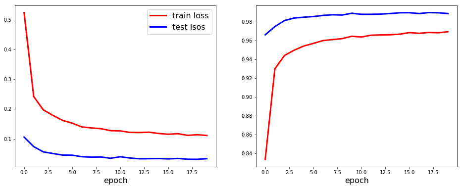
まずはじめに、動的ではない(静的な)グラフの例を示します。手書き数字認識のような識別タスクにおいて、最も一般的であると思われる評価尺度として、ロスと正解率を可視化します。train_loop関数は、返り値にロスと正解率のhistoryを返すようにしたので、それを使ってグラフを作ります。
図の作成にはいろんなツールがあると思うのですが、matplotlibが定番で(僕は)大きな不満もないので、よく使っています。
model = Net().cuda() if use_cuda else Net()
optimizer = optim.Adadelta(model.parameters())
history = train_loop(model, data_loaders, optimizer, epochs)
print("Test loss: {:.3f}".format(history["train"]["loss"][-1]))
print("Test acc: {:.3f}".format(history["test"]["acc"][-1]))
Test loss: 0.111
Test acc: 0.989
matplotlib.pyplot.figure(figsize=(16,6))
subplot(1,2,1)
plot(history["train"]["loss"], linewidth=3, color="red", label="train loss")
plot(history["test"]["loss"], linewidth=3, color="blue", label="test lsos")
xlabel("epoch", fontsize=16)
legend(prop={"size": 16})
subplot(1,2,2)
plot(history["train"]["acc"], linewidth=3, color="red", label="train acc")
plot(history["test"]["acc"], linewidth=3, color="blue", label="test acc")
xlabel("epoch", fontsize=16)
<matplotlib.text.Text at 0x7f16fa9ca438>
1. Line
次に、上記の線グラフを、Bokehを使って作ってみます。これには、 https://bokeh.pydata.org/en/latest/docs/reference/models/glyphs/line.html が使えます。
bokehで作ったグラフをnotebookにinline plotするためには、bokeh.io.output_notebook を呼び出しておく必要があります。
import bokeh
import bokeh.io
from bokeh.io import push_notebook, show, output_notebook
from bokeh.plotting import figure
try:
    # 少し古いbokehだとこっち
    from bokeh.io import gridplot
except ImportError:
    from bokeh.layouts import gridplot

output_notebook()
次に定義する LinePlotsCallback は、グラフの情報をプロパティに保持し、on_epoch_end で学習結果のhisotoryを受け取って、ロスと正解率のグラフを更新します。 historyには、今回の場合は、
- ロス (float)
- 正解率 (float)
- カテゴリ毎の総サンプル数 (list)
- カテゴリ毎の正解サンプル数 (list)
の4つを含めるように実装しました (train_loop 関数を参照)。LinePlotsCallback では、このうちロスと正解率を随時受け取って、グラフを更新します。Line オブジェクトの更新には、data_source.data["x"], data_source.data["y"] に随時値を追加していくことで行います。
以降示すグラフでも同じなのですが、グラフを生成する基本的な手順をまとめると、
- bokeh.plotting.figure により、figureオブジェクトを生成する
- 生成したfigureオブジェクトに対して、線グラフ、棒グラフといったパーツ (レンダラ、bokehではglyphsと呼ぶ) を生成する
- (今回は格子状に図を配置したかったので)複数のfigureオブジェクトをgrid上にレイアウトする
となっています。格子状に配置しない場合は最後のステップは不要ですが、便利なので使います。
グラフの更新は、レンダラに値をセットしたあとに、bokeh.io.push_notebook を呼び出すことで行います。
class LinePlotsCallback(object):
    def __init__(self, epochs=epochs, batch_size=batch_size):
        # Epoch毎
        p1 = figure(title="Loss", plot_height=300, plot_width=350,
                        y_range=(0, 0.5), x_range=(-1, epochs+1))
        p2 = figure(title="Acc", plot_height=300, plot_width=350,
                        y_range=(0.8, 1.0), x_range=(-1, epochs+1))

        self.renderers = {"train":{}, "test":{}}

        # 赤: train, 青: テスト
        for phase, c in [("train", "red"), ("test", "blue")]:
            for (p, key) in [(p1, "loss"), (p2, "acc")]:
                self.renderers[phase][key] = p.line([], [], color=c, line_width=3)

        self.graph = gridplot([p1, p2], ncols=2, toolbar_location=toolbar_location)


    def on_epoch_end(self, epoch, phase, history):
        for key in ["loss", "acc"]:
            self.renderers[phase][key].data_source.data["x"].append(epoch)
            self.renderers[phase][key].data_source.data["y"].append(history[phase][key][-1])
        push_notebook()
        if save_img:
            bokeh.io.export_png(self.graph, "fig/{:02d}_line.png".format(epoch))
callback = LinePlotsCallback()
if show_static:
    if exists("fig/line.gif"):
        with open("fig/line.gif", 'rb') as f:
            IPython.display.display(Image(data=f.read()), format="gif")
else:
    bokeh.io.show(callback.graph, notebook_handle=True)
model = Net().cuda() if use_cuda else Net()
optimizer = optim.Adadelta(model.parameters())
history = train_loop(model, data_loaders, optimizer, epochs, callback=callback)
print("Test loss: {:.3f}".format(history["train"]["loss"][-1]))
print("Test acc: {:.3f}".format(history["test"]["acc"][-1]))
Test loss: 0.113
Test acc: 0.990
2. VBar
データセット全体の正解率だけでなく、カテゴリ毎の正解率などの尺度を知りたい時がよくあります。次は、数字の各カテゴリごとにどのくらい正解しているのか、といった尺度を可視化するために、縦棒グラフを作ってみます。これには、 https://bokeh.pydata.org/en/latest/docs/reference/models/glyphs/vbar.html が使えます。on_epoch_endで渡されるhistoryのうち、
- カテゴリ毎の総サンプル数 (list)
- カテゴリ毎の正解サンプル数 (list)
の二つを使って動的にグラフを更新します。
Line オブジェクトの更新は、data_source.data["x"], data_source.data["y"] に値を追加していくことで行いましたが、VBarオブジェクトの場合は、data_source.data["top"] に値をセットします。下向きの棒グラフが作りたい場合は、data_source.data["bottom"] に値をセットすればOKです。
class VBarPlotsCallback(object):
    def __init__(self, epochs=epochs, batch_size=batch_size):
        # Epoch毎
        p1 = figure(title="Category-wise correctness (train)",
                    plot_height=300, plot_width=350, y_range=(0, 7000))
        p2 = figure(title="Category-wise correctness (test)",
                    plot_height=300, plot_width=350, y_range=(0, 1500))

        self.renderers = {"train":{}, "test":{}}

        bar_opts = dict(width=0.8, alpha=0.5)
        for phase, p in [("train", p1), ("test", p2)]:
            for (key, c) in [("corrects", "blue"), ("counts", "red")]:
                self.renderers[phase][key] = p.vbar(
                    x=np.arange(0,10), top=[0]*10, name="test", color=c, **bar_opts)

        self.graph = gridplot([p1, p2], ncols=2, toolbar_location=toolbar_location)

    def on_epoch_end(self, epoch, phase, history):
        for key in ["counts", "corrects"]:
            self.renderers[phase][key].data_source.data["top"] = history[phase][key][-1]
            push_notebook()
        if save_img:
            bokeh.io.export_png(self.graph, "fig/{:02d}_vbar.png".format(epoch))
callback = VBarPlotsCallback()
if show_static:
    if exists("fig/vbar.gif"):
        with open("fig/vbar.gif", 'rb') as f:
            IPython.display.display(Image(data=f.read()), format="gif")
else:
    bokeh.io.show(callback.graph, notebook_handle=True)
model = Net().cuda() if use_cuda else Net()
optimizer = optim.Adadelta(model.parameters())
history = train_loop(model, data_loaders, optimizer, epochs, callback=callback)
print("Test loss: {:.3f}".format(history["train"]["loss"][-1]))
print("Test acc: {:.3f}".format(history["test"]["acc"][-1]))
Test loss: 0.115
Test acc: 0.989
3. HBar
HBarと非常に似たグラフとして、横向きの棒グラフである https://bokeh.pydata.org/en/latest/docs/reference/models/glyphs/hbar.html があります。VBarの場合と同様に、カテゴリ毎の正解サンプル数を可視化してみます。本質的に可視化する情報は変わりませんが、あくまでデモということで。
HBarオブジェクトの更新は、data_source.data["right"] or data_source.data["left"] に値をセットすればOKです。
class HBarPlotsCallback(object):
    def __init__(self, epochs=epochs, batch_size=batch_size):
        # Epoch毎
        p1 = figure(title="Category-wise correctness (train)",
                    plot_height=300, plot_width=350, x_range=(0, 7000))
        p2 = figure(title="Category-wise correctness (test)",
                    plot_height=300, plot_width=350, x_range=(0, 1500))

        self.renderers = {"train":{}, "test":{}}

        bar_opts = dict(height=0.8, alpha=0.5)
        for phase, p in [("train", p1), ("test", p2)]:
            for (key, c) in [("corrects", "blue"), ("counts", "green")]:
                self.renderers[phase][key] = p.hbar(
                    y=np.arange(0,10), right=[0]*10, name="test", color=c, **bar_opts)

        self.graph = gridplot([p1, p2], ncols=2, toolbar_location=toolbar_location)

    def on_epoch_end(self, epoch, phase, history):
        for key in ["counts", "corrects"]:
            self.renderers[phase][key].data_source.data["right"] = history[phase][key][-1]
            push_notebook()
        if save_img:
            bokeh.io.export_png(self.graph, "fig/{:02d}_hbar.png".format(epoch))
callback = HBarPlotsCallback()
if show_static:
    if exists("fig/hbar.gif"):
        with open("fig/hbar.gif", 'rb') as f:
            IPython.display.display(Image(data=f.read()), format="gif")
else:
    bokeh.io.show(callback.graph, notebook_handle=True)
model = Net().cuda() if use_cuda else Net()
optimizer = optim.Adadelta(model.parameters())
history = train_loop(model, data_loaders, optimizer, epochs, callback=callback)
print("Test loss: {:.3f}".format(history["train"]["loss"][-1]))
print("Test acc: {:.3f}".format(history["test"]["acc"][-1]))
Test loss: 0.116
Test acc: 0.989
5. Image
最後に、https://bokeh.pydata.org/en/latest/docs/reference/models/glyphs/image_rgba.html を使って、画像を可視化する例を紹介します。例えば生成モデルを学習するときなど、学習の過程で、その生成サンプルを可視化したい場合がよくあるので、そういった場合に使えます。
最初に実装したモデルは手書き数字認識のための識別モデルだったため、趣向を変えて、生成モデルである Variational Auto-encoder (VAE) を使います。識別モデルの学習と生成モデルの学習は少し毛色が違うので、(ほとんど同じですが、簡単のため)併せて学習用のコードを書き換えました。
VAE
https://github.com/pytorch/examples/tree/master/vae
class VAE(nn.Module):
    def __init__(self):
        super(VAE, self).__init__()

        self.fc1 = nn.Linear(784, 400)
        self.fc21 = nn.Linear(400, 20)
        self.fc22 = nn.Linear(400, 20)
        self.fc3 = nn.Linear(20, 400)
        self.fc4 = nn.Linear(400, 784)

        self.relu = nn.ReLU()
        self.sigmoid = nn.Sigmoid()

    def encode(self, x):
        h1 = self.relu(self.fc1(x))
        return self.fc21(h1), self.fc22(h1)

    def reparameterize(self, mu, logvar):
        if self.training:
            std = logvar.mul(0.5).exp_()
            eps = Variable(std.data.new(std.size()).normal_())
            return eps.mul(std).add_(mu)
        else:
            return mu

    def decode(self, z):
        h3 = self.relu(self.fc3(z))
        return self.sigmoid(self.fc4(h3))

    def forward(self, x):
        mu, logvar = self.encode(x.view(-1, 784))
        z = self.reparameterize(mu, logvar)
        return self.decode(z), mu, logvar

def loss_function(recon_x, x, mu, logvar):
    BCE = F.binary_cross_entropy(recon_x, x.view(-1, 784))

    # see Appendix B from VAE paper:
    # Kingma and Welling. Auto-Encoding Variational Bayes. ICLR, 2014
    # https://arxiv.org/abs/1312.6114
    # 0.5 * sum(1 + log(sigma^2) - mu^2 - sigma^2)
    KLD = -0.5 * torch.sum(1 + logvar - mu.pow(2) - logvar.exp())
    # Normalise by same number of elements as in reconstruction
    KLD /= batch_size * 784

    return BCE + KLD
Training loop
def __train_loop_vae(model, data_loaders, optimizer, epoch, phase):
    model = model.train() if phase == "train" else model.eval()
    running_loss = 0
    recon_batch_first, target = None, None
    for batch_idx, (x, _) in enumerate(data_loaders[phase]):
        x = x.cuda() if use_cuda else x
        x = Variable(x)
        optimizer.zero_grad()
        y_hat = model(x)

        # loss
        recon_batch, mu, logvar = model(x)
        loss = loss_function(recon_batch, x, mu, logvar)

        # update
        if phase == "train":
            loss.backward()
            optimizer.step()
        running_loss += loss.data[0]

        if target is None:
            target = x
            recon_batch_first = recon_batch

    # epoch-wise metrics
    l = running_loss / len(data_loaders[phase])
    return {"loss": l, "recon": recon_batch_first.data.cpu(), "target": target.data.cpu()}

def train_loop_vae(model, data_loaders, optimizer, epochs=12, callback=None):
    history = {"train": {}, "test": {}}
    for epoch in tnrange(epochs):
        for phase in ["train", "test"]:
            d = __train_loop_vae(model, data_loaders, optimizer, epoch, phase)
            for k,v in d.items():
                try:
                    history[phase][k].append(v)
                except KeyError:
                    history[phase][k] = [v]

            if callback is not None:
                callback.on_epoch_end(epoch, phase, history)
    return history
さて、準備は終わりです。
次に示す ImagePlotsCallback は、on_epoch_end で学習結果のhisotoryを受け取って、VAEを通して復元した画像と、復元したい対象の画像を動的に更新します。ImageRGBA の場合は、data_source.data["image"] に配列をセットすることで、更新することができます。
注意事項として、モノクロ画像を描画する際には、適当なカラーマップをかけて、(w, h) -> (w, h, 4) の配列にしておく必要があります。
from torchvision.utils import make_grid
from matplotlib.pyplot import cm

def _to_img(batch, cmap=cm.gray):
    # 128は多かったので半分にします
    _batch_size = batch_size // 2
    batch = batch[:_batch_size]

    batch = batch.view(-1,1,28,28)
    grid = make_grid(batch, nrow=int(np.sqrt(_batch_size)))[0].numpy()
    # Force squared
    l = np.min(grid.shape)
    grid = grid[:l, :l]
    img = np.uint8(cmap(grid) * 255)
    return img

class ImagePlotsCallback(object):
    def __init__(self, epochs=epochs, batch_size=batch_size, cmap=cm.gray):
        x_range, y_range = (-0.5, 10.5), (-0.5, 10.5)
        p1 = figure(title="Reconstructed (train)",
                    plot_height=350, plot_width=350, x_range=x_range, y_range=y_range)
        p2 = figure(title="Target (train)",
                    plot_height=350, plot_width=350, x_range=x_range, y_range=y_range)
        p3 = figure(title="Reconstructed (test)",
                    plot_height=350, plot_width=350, x_range=x_range, y_range=y_range)
        p4 = figure(title="Target (test)",
                    plot_height=350, plot_width=350, x_range=x_range, y_range=y_range)
        self.cmap = cmap

        self.renderers = {"train":{}, "test":{}}
        empty = torch.zeros(batch_size,1,28,28)
        empty = _to_img(empty, self.cmap)
        # to adjast aspect ratio
        r = empty.shape[0]/empty.shape[1]

        # https://github.com/bokeh/bokeh/issues/1666
        for k, p in [("recon", p1), ("target", p2)]:
            self.renderers["train"][k] = p.image_rgba(image=[empty[::-1]], x=[0], y=[0], dw=[10], dh=[r*10])
        for k, p in [("recon", p3), ("target", p4)]:
            self.renderers["test"][k] = p.image_rgba(image=[empty[::-1]], x=[0], y=[0], dw=[10], dh=[r*10])

        self.graph = gridplot([p1, p2, p3, p4], ncols=2, toolbar_location=toolbar_location)

    def on_epoch_end(self, epoch, phase, history):
        for k in ["recon", "target"]:
            self.renderers[phase][k].data_source.data["image"] = [_to_img(history[phase][k][-1], self.cmap)[::-1]]
        push_notebook()

        if save_img:
            bokeh.io.export_png(self.graph, "fig/{:02d}_{}_image.png".format(epoch, self.cmap.name))
# グレースケール
callback = ImagePlotsCallback(cmap=cm.gray)
if show_static:
    if exists("fig/gray_image.gif"):
        with open("fig/gray_image.gif", 'rb') as f:
            IPython.display.display(Image(data=f.read()), format="gif")
else:
    bokeh.io.show(callback.graph, notebook_handle=True)

# gifを作ったときに見やすいように、shuffle=Falseにする
kwargs = {'num_workers': 1, 'pin_memory': True} if use_cuda else {}
train_loader = torch.utils.data.DataLoader(
    datasets.MNIST('./data', train=True, download=True,
                   transform=transforms.Compose([
                       transforms.ToTensor()
                   ])),
    batch_size=batch_size, shuffle=False, **kwargs)
test_loader = torch.utils.data.DataLoader(
    datasets.MNIST('./data', train=False, transform=transforms.Compose([
                       transforms.ToTensor(),
                   ])),
    batch_size=batch_size, shuffle=False, **kwargs)

data_loaders = {"train": train_loader, "test":test_loader}
model = VAE().cuda() if use_cuda else VAE()
optimizer = optim.Adam(model.parameters(), lr=1e-3)
history = train_loop_vae(model, data_loaders, optimizer, epochs, callback=callback)
print("Test loss: {:.3f}".format(history["train"]["loss"][-1]))
Test loss: 0.133
本質的な違いはありませんが、異なるカラーマップを試してみます。
gradient = np.linspace(0,1,256)
gradient = np.vstack((gradient, gradient))
pyplot.figure(figsize=(16,0.5))
imshow(gradient, aspect="auto", cmap=cm.inferno)
axis("off");

callback = ImagePlotsCallback(cmap=cm.inferno)
if show_static:
    if exists("fig/inferno_image.gif"):
        with open("fig/inferno_image.gif", 'rb') as f:
            IPython.display.display(Image(data=f.read()), format="gif")
else:
    bokeh.io.show(callback.graph, notebook_handle=True)
model = VAE().cuda() if use_cuda else VAE()
optimizer = optim.Adam(model.parameters(), lr=1e-3)
history = train_loop_vae(model, data_loaders, optimizer, epochs, callback=callback)
print("Test loss: {:.3f}".format(history["train"]["loss"][-1]))
Test loss: 0.133
おわりに
Bokehによるグラフ作成は、少しとっつきにくいかもしれませんが(matplotlibとかではレンダラとか意識しないですよね)、慣れれば柔軟性が高く、便利なのではないかと思います。
今回の記事を書くにあたっては、bokeh v0.12.9 を使いました。もしローカルでnotebookを実行する場合は、バージョンを揃えることをおすすめします。
参考
Ryuichi Yamamoto
Engineer/Researcher
I am a engineer/researcher passionate about speech synthesis. I love to write code and enjoy open-source collaboration on GitHub. Please feel free to reach out on Twitter and GitHub.