第5章深層学習に基づく統計的パラメトリック音声合成¶

準備¶

Python version¶

[1]:

!python -VV

Python 3.8.6 | packaged by conda-forge | (default, Dec 26 2020, 05:05:16)
[GCC 9.3.0]

ttslearn のインストール¶

[2]:

%%capture
try:
    import ttslearn
except ImportError:
    !pip install ttslearn

[3]:

import ttslearn
ttslearn.__version__

[3]:

'0.2.1'

パッケージのインポート¶

[4]:

%pylab inline
%load_ext autoreload
%autoreload
import IPython
from IPython.display import Audio
import os
import numpy as np
import torch
import librosa
import librosa.display

Populating the interactive namespace from numpy and matplotlib

[5]:

# シードの固定
from ttslearn.util import init_seed
init_seed(1234)

描画周りの設定¶

[6]:

from ttslearn.notebook import get_cmap, init_plot_style, savefig
cmap = get_cmap()
init_plot_style()

5.3 フルコンテキストラベルとは？¶

モノフォンラベル¶

[7]:

from nnmnkwii.io import hts
import ttslearn
from os.path import basename

labels = hts.load(ttslearn.util.example_label_file(mono=True))
print(labels[:6])

0 3125000 sil
3125000 3525000 m
3525000 4325000 i
4325000 5225000 z
5225000 5525000 u
5525000 6525000 o

[8]:

# 秒単位に変換
# NOTE: 100ナノ秒単位: 100 * 1e-9 = 1e-7
for s,e,l in labels[:6]:
    print(s*1e-7, e*1e-7, l)

0.0 0.3125 sil
0.3125 0.3525 m
0.3525 0.4325 i
0.4325 0.5225 z
0.5225 0.5525 u
0.5525 0.6525 o

フルコンテキストラベル¶

[9]:

labels = hts.load(ttslearn.util.example_label_file(mono=False))
for start_time, end_time, context in labels[:6]:
    print(f"{start_time} {end_time} {context}")

0 3125000 xx^xx-sil+m=i/A:xx+xx+xx/B:xx-xx_xx/C:xx_xx+xx/D:02+xx_xx/E:xx_xx!xx_xx-xx/F:xx_xx#xx_xx@xx_xx|xx_xx/G:3_3%0_xx_xx/H:xx_xx/I:xx-xx@xx+xx&xx-xx|xx+xx/J:5_23/K:1+5-23
3125000 3525000 xx^sil-m+i=z/A:-2+1+3/B:xx-xx_xx/C:02_xx+xx/D:13+xx_xx/E:xx_xx!xx_xx-xx/F:3_3#0_xx@1_5|1_23/G:7_2%0_xx_1/H:xx_xx/I:5-23@1+1&1-5|1+23/J:xx_xx/K:1+5-23
3525000 4325000 sil^m-i+z=u/A:-2+1+3/B:xx-xx_xx/C:02_xx+xx/D:13+xx_xx/E:xx_xx!xx_xx-xx/F:3_3#0_xx@1_5|1_23/G:7_2%0_xx_1/H:xx_xx/I:5-23@1+1&1-5|1+23/J:xx_xx/K:1+5-23
4325000 5225000 m^i-z+u=o/A:-1+2+2/B:xx-xx_xx/C:02_xx+xx/D:13+xx_xx/E:xx_xx!xx_xx-xx/F:3_3#0_xx@1_5|1_23/G:7_2%0_xx_1/H:xx_xx/I:5-23@1+1&1-5|1+23/J:xx_xx/K:1+5-23
5225000 5525000 i^z-u+o=m/A:-1+2+2/B:xx-xx_xx/C:02_xx+xx/D:13+xx_xx/E:xx_xx!xx_xx-xx/F:3_3#0_xx@1_5|1_23/G:7_2%0_xx_1/H:xx_xx/I:5-23@1+1&1-5|1+23/J:xx_xx/K:1+5-23
5525000 6525000 z^u-o+m=a/A:0+3+1/B:02-xx_xx/C:13_xx+xx/D:18+xx_xx/E:xx_xx!xx_xx-xx/F:3_3#0_xx@1_5|1_23/G:7_2%0_xx_1/H:xx_xx/I:5-23@1+1&1-5|1+23/J:xx_xx/K:1+5-23

5.4 言語特徴量の抽出¶

Open JTalk による言語特徴量の抽出¶

[10]:

import pyopenjtalk

pyopenjtalk.g2p("今日もいい天気ですね", kana=True)

[10]:

'キョーモイイテンキデスネ'

[11]:

pyopenjtalk.g2p("今日もいい天気ですね", kana=False)

[11]:

'ky o o m o i i t e N k i d e s U n e'

[12]:

labels = pyopenjtalk.extract_fullcontext("今日")
for label in labels:
    print(label)

xx^xx-sil+ky=o/A:xx+xx+xx/B:xx-xx_xx/C:xx_xx+xx/D:xx+xx_xx/E:xx_xx!xx_xx-xx/F:xx_xx#xx_xx@xx_xx|xx_xx/G:2_1%0_xx_xx/H:xx_xx/I:xx-xx@xx+xx&xx-xx|xx+xx/J:1_2/K:1+1-2
xx^sil-ky+o=o/A:0+1+2/B:xx-xx_xx/C:02_xx+xx/D:xx+xx_xx/E:xx_xx!xx_xx-xx/F:2_1#0_xx@1_1|1_2/G:xx_xx%xx_xx_xx/H:xx_xx/I:1-2@1+1&1-1|1+2/J:xx_xx/K:1+1-2
sil^ky-o+o=sil/A:0+1+2/B:xx-xx_xx/C:02_xx+xx/D:xx+xx_xx/E:xx_xx!xx_xx-xx/F:2_1#0_xx@1_1|1_2/G:xx_xx%xx_xx_xx/H:xx_xx/I:1-2@1+1&1-1|1+2/J:xx_xx/K:1+1-2
ky^o-o+sil=xx/A:1+2+1/B:xx-xx_xx/C:02_xx+xx/D:xx+xx_xx/E:xx_xx!xx_xx-xx/F:2_1#0_xx@1_1|1_2/G:xx_xx%xx_xx_xx/H:xx_xx/I:1-2@1+1&1-1|1+2/J:xx_xx/K:1+1-2
o^o-sil+xx=xx/A:xx+xx+xx/B:xx-xx_xx/C:xx_xx+xx/D:xx+xx_xx/E:2_1!0_xx-xx/F:xx_xx#xx_xx@xx_xx|xx_xx/G:xx_xx%xx_xx_xx/H:1_2/I:xx-xx@xx+xx&xx-xx|xx+xx/J:xx_xx/K:1+1-2

HTS 形式の質問ファイル¶

[13]:

qst_path = ttslearn.util.example_qst_file()
! cat $qst_path | grep QS | head -1
! cat $qst_path | grep CQS | head -1

QS "L-Phone_A"   {*^A-*}
CQS "a1-C-Accent_Diff"                  {A:([-\d]+)+}

[14]:

! head {ttslearn.util.example_qst_file()}

QS "L-Phone_A"   {*^A-*}
QS "L-Phone_E"   {*^E-*}
QS "L-Phone_I"   {*^I-*}
QS "L-Phone_N"   {*^N-*}
QS "L-Phone_O"   {*^O-*}
QS "L-Phone_U"   {*^U-*}
QS "L-Phone_a"   {*^a-*}
QS "L-Phone_b"   {*^b-*}
QS "L-Phone_by"  {*^by-*}
QS "L-Phone_ch"  {*^ch-*}

[15]:

! tail {ttslearn.util.example_qst_file()}

CQS "i1-C-Breath_Phrase_Num"            {/I:(\d+)-}
CQS "i2-C-Breath_Mora_Num"              {-(\d+)@}
CQS "i3-C-Breath_Pos_Forward"           {@(\d+)+}
CQS "i4-C-Breath_Pos_Backward"          {+(\d+)&}
CQS "i5-C-Breath_Accent_Pos_Forward"    {&(\d+)-}
CQS "i6-C-Breath_Accent_Pos_Backward"   {-(\d+)|}
CQS "i7-C-Breath_Mora_Pos_Forward"      {|(\d+)+}
CQS "i8-C-Breath_Mora_Pos_Backward"     {+(\d+)/J:}
CQS "j1-R-Breath_Phrase_Num"            {/J:(\d+)_}
CQS "j2-R-Breath_Mora_Num"              {_(\d+)/K:}

HTS 形式の質問ファイルの読み込み¶

[16]:

from nnmnkwii.io import hts
import ttslearn

binary_dict, numeric_dict = hts.load_question_set(ttslearn.util.example_qst_file())

# 1番目の質問を確認します
name, ex = binary_dict[0]
print("二値特徴量の数:", len(binary_dict))
print("数値特徴量の数:", len(numeric_dict))
print("1 つ目の質問:", name, ex)

二値特徴量の数: 300
数値特徴量の数: 25
1 つ目の質問: L-Phone_A [re.compile('\\^A\\-')]

フルコンテキストラベルからの数値表現への変換¶

[17]:

from nnmnkwii.frontend import merlin as fe

labels = hts.load(ttslearn.util.example_label_file())
feats = fe.linguistic_features(labels, binary_dict, numeric_dict)
print("言語特徴量（音素単位）のサイズ:", feats.shape)

言語特徴量（音素単位）のサイズ: (44, 325)

[18]:

feats

[18]:

array([[ 0.,  0.,  0., ..., -1.,  5., 23.],
       [ 0.,  0.,  0., ..., 23., -1., -1.],
       [ 0.,  0.,  0., ..., 23., -1., -1.],
       ...,
       [ 0.,  0.,  0., ..., 23., -1., -1.],
       [ 0.,  0.,  0., ..., 23., -1., -1.],
       [ 0.,  0.,  0., ..., -1., -1., -1.]])

言語特徴量をフレーム単位に展開¶

[19]:

feats_phoneme = fe.linguistic_features(labels, binary_dict, numeric_dict, add_frame_features=False)
feats_frame = fe.linguistic_features(labels, binary_dict, numeric_dict, add_frame_features=True)
print("言語特徴量（音素単位）のサイズ:", feats_phoneme.shape)
print("言語特徴量（フレーム単位）のサイズ:", feats_frame.shape)

言語特徴量（音素単位）のサイズ: (44, 325)
言語特徴量（フレーム単位）のサイズ: (636, 325)

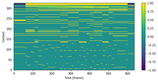
言語特徴量の可視化 (bonus)¶

[20]:

# 可視化用に正規化
in_feats = feats_frame / np.maximum(1, np.abs(feats_frame).max(0))
fig, ax = plt.subplots(figsize=(8,4))
mesh = ax.imshow(in_feats.T, aspect="auto", interpolation="none", origin="lower", cmap=cmap)
fig.colorbar(mesh, ax=ax)

ax.set_xlabel("Time [frame]")
ax.set_ylabel("Context")
plt.tight_layout()

../_images/notebooks_ch05_DNNTTS_35_0.png

5.5 音響特徴量の抽出¶

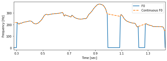
対数基本周波数¶

[21]:

from scipy.io import wavfile
import pyworld
from nnmnkwii.preprocessing.f0 import interp1d

# 基本周波数を対数基本周波数へ変換する関数
def f0_to_lf0(f0):
    lf0 = f0.copy()
    nonzero_indices = np.nonzero(f0)
    lf0[nonzero_indices] = np.log(f0[nonzero_indices])
    return lf0

# 音声ファイルの読み込み
sr, x = wavfile.read(ttslearn.util.example_audio_file())
x = x.astype(np.float64)

# DIO による基本周波数推定
f0, timeaxis = pyworld.dio(x, sr)

# 基本周波数を対数基本周波数に変換
lf0 = f0_to_lf0(f0)

# 対数基本周波数に対して線形補間
clf0 = interp1d(lf0, kind="linear")

# 可視化
fig, ax = plt.subplots(figsize=(8, 3))
ax.plot(timeaxis, np.exp(lf0), linewidth=2, label="F0")
ax.plot(timeaxis, np.exp(clf0), "--", linewidth=2, label="Continuous F0")
ax.set_xlabel("Time [sec]")
ax.set_xticks(np.arange(0.3, 1.4, 0.2))
ax.set_xlim(0.28, 1.43)
ax.set_ylabel("Frequency [Hz]")
ax.legend()
plt.tight_layout()

# 図5-6
savefig("fig/dnntts_cf0")

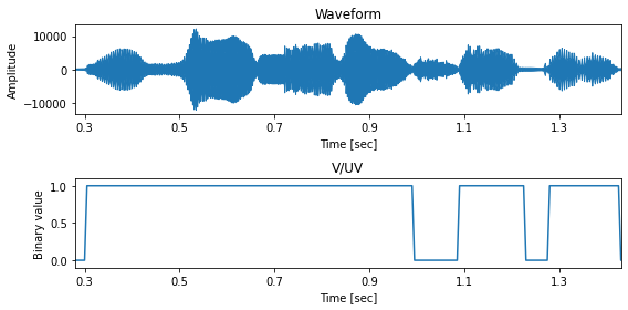
../_images/notebooks_ch05_DNNTTS_38_0.png

有声/無声フラグ¶

[22]:

# DIO による基本周波数推定
f0, timeaxis = pyworld.dio(x, sr)

# 有声/無声フラグ の計算
vuv = (f0 > 0).astype(np.float32)

hop_length = int(sr * 0.005)
fig, ax = plt.subplots(2, 1, figsize=(8,4))
librosa.display.waveplot(x, sr=sr, x_axis="time", ax=ax[0])
ax[1].plot(timeaxis, vuv)
ax[1].set_ylim(-0.1, 1.1)

ax[0].set_title("Waveform")
ax[1].set_title("V/UV")
ax[0].set_xlabel("Time [sec]")
ax[0].set_ylabel("Amplitude")
ax[1].set_xlabel("Time [sec]")
ax[1].set_ylabel("Binary value")

for a in ax:
    a.set_xlim(0.28, 1.43)
    a.set_xticks(np.arange(0.3, 1.4, 0.2))
plt.tight_layout()

# 図5-7
savefig("fig/dnntts_vuv")

../_images/notebooks_ch05_DNNTTS_40_0.png

メルケプストラム¶

[23]:

import pysptk

# DIO による基本周波数の推定
f0, timeaxis = pyworld.dio(x, sr)

# CheapTrick によるスペクトル包絡の推定
# 返り値は、パワースペクトルであることに注意 (振幅が 2 乗されている)
spectrogram = pyworld.cheaptrick(x, f0, timeaxis, sr)

# 線形周波数軸をメル周波数尺度に伸縮し、その後ケプストラムに変換
# alpha は周波数軸の伸縮のパラメータを表します
alpha = pysptk.util.mcepalpha(sr)
# FFT 長は、サンプリング周波数が 48kHz の場合は 2048
fftlen = pyworld.get_cheaptrick_fft_size(sr)
# メルケプストラムの次元数は、 mgc_order + 1 となります
# NOTE: メル一般化ケプストラム (Mel-generalized cepstrum) の頭文字を取り、
# 変数名を mgc とします
mgc_order = 59
mgc = pysptk.sp2mc(spectrogram, mgc_order, alpha)

# メルケプストラムから元のスペクトル包絡を復元
# スペクトルの次元数は、　fftlen//2 + 1 = 1025
spectrogram_reconstructed = pysptk.mc2sp(mgc, alpha, fftlen)

# 可視化
hop_length = int(sr * 0.005)
fig, ax = plt.subplots(3, 1, figsize=(8,8))
ax[0].set_title("Mel-cepstrum")
ax[1].set_title("Reconstructed spectral envelope from Mel-cepstrum")
ax[2].set_title("Spectral envelope of natural speech")

mesh = librosa.display.specshow(mgc.T, sr=sr, hop_length=hop_length, x_axis="time", cmap=cmap, ax=ax[0])
fig.colorbar(mesh, ax=ax[0])
ax[0].set_yticks(np.arange(mgc_order+2)[::10])

log_sp_reconstructed = librosa.power_to_db(np.abs(spectrogram_reconstructed), ref=np.max)
mesh = librosa.display.specshow(log_sp_reconstructed.T, sr=sr, hop_length=hop_length, x_axis="time", y_axis="hz", cmap=cmap, ax=ax[1])
fig.colorbar(mesh, ax=ax[1], format="%+2.f dB")

log_sp = librosa.power_to_db(np.abs(spectrogram), ref=np.max)
mesh = librosa.display.specshow(log_sp.T, sr=sr, hop_length=hop_length, x_axis="time", y_axis="hz", cmap=cmap, ax=ax[2])
fig.colorbar(mesh, ax=ax[2], format="%+2.f dB")

ax[1].set_ylim(0, 12000)
ax[2].set_ylim(0, 12000)

for a in ax:
    a.set_xlabel("Time [sec]")
    a.set_xlim(0.28, 1.43)
    a.set_xticks(np.arange(0.3, 1.4, 0.2))

ax[0].set_ylabel("Mel channel")
ax[1].set_ylabel("Frequency [Hz]")
ax[2].set_ylabel("Frequency [Hz]")

plt.tight_layout()

# 図5-8
savefig("fig/dnntts_mcep_reconstructed")

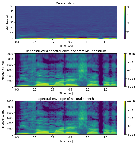
../_images/notebooks_ch05_DNNTTS_42_0.png

[24]:

print("圧縮率:", spectrogram.shape[1]/mgc.shape[1])

圧縮率: 17.083333333333332

帯域非周期性指標¶

[25]:

# DIO による基本周波数の推定
f0, timeaxis = pyworld.dio(x, sr)

# D4C による非周期性指標の推定
aperiodicity= pyworld.d4c(x, f0, timeaxis, sr)

# 帯域別の非周期性指標に圧縮
bap = pyworld.code_aperiodicity(aperiodicity, sr)

# 可視化
hop_length = int(sr * 0.005)
fig, ax = plt.subplots(2, 1, figsize=(8,6))
mesh = librosa.display.specshow(20*np.log10(aperiodicity).T, sr=sr, hop_length=hop_length, x_axis="time", y_axis="linear", cmap=cmap, ax=ax[0])
ax[0].set_title("Aperiodicity")
fig.colorbar(mesh, ax=ax[0], format="%+2.f dB")

mesh = librosa.display.specshow(bap.T, sr=sr, hop_length=hop_length, x_axis="time", cmap=cmap, ax=ax[1])
fig.colorbar(mesh, ax=ax[1], format="%+2.f dB")
ax[1].set_title("Band-aperiodicity")
for a in ax:
    a.set_xlabel("Time [sec]")
    a.set_ylabel("Frequency [Hz]")
    a.set_xlim(0.28, 1.43)
    a.set_xticks(np.arange(0.3, 1.4, 0.2))

ax[1].set_yticks(np.arange(5+1))
ax[1].set_ylabel("Frequency band")
plt.tight_layout()

# 図5-9
savefig("fig/dnntts_bap")

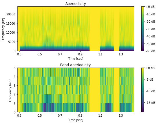
../_images/notebooks_ch05_DNNTTS_45_0.png

[26]:

print("圧縮率:", aperiodicity.shape[1]/bap.shape[1])

圧縮率: 205.0

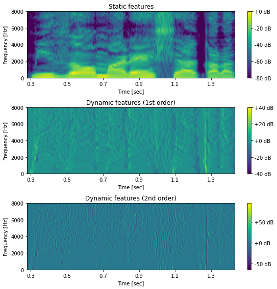
動的特徴量¶

[27]:

def compute_delta(x, w):
    y = np.zeros_like(x)
    # 特徴量の次元ごとに動的特徴量を計算
    for d in range(x.shape[1]):
        y[:, d] = np.correlate(x[:, d], w, mode="same")
    return y

[28]:

import librosa

# スペクトル包絡の推定
f0, timeaxis = pyworld.dio(x, sr)
spectrogram = pyworld.cheaptrick(x, f0, timeaxis, sr)

# パワースペクトルを対数に変換
spectrogram = librosa.power_to_db(spectrogram, ref=np.max)

# 動的特徴量の計算
delta_window1 = [-0.5, 0.0, 0.5] # 1 次動的特徴量に対する窓
delta_window2 = [1.0, -2.0, 1.0] # 2 次動的特徴量に対する窓

# 1 次動的特徴量
delta = compute_delta(spectrogram, delta_window1)

# 2 次動的特徴量
deltadelta = compute_delta(spectrogram, delta_window2)

# スペクトル包絡に対して動的特徴量を計算して可視化
hop_length = int(sr * 0.005)
fig, ax = plt.subplots(3, 1, figsize=(8,8))
ax[0].set_title("Static features")
ax[1].set_title("Dynamic features (1st order)")
ax[2].set_title("Dynamic features (2nd order)")
mesh = librosa.display.specshow(spectrogram.T, sr=sr, hop_length=hop_length, x_axis="time", y_axis="hz", cmap=cmap, ax=ax[0])
fig.colorbar(mesh, ax=ax[0], format="%+2.f dB")
mesh = librosa.display.specshow(delta.T, sr=sr, hop_length=hop_length, x_axis="time", y_axis="hz", cmap=cmap, ax=ax[1])
fig.colorbar(mesh, ax=ax[1], format="%+2.f dB")
mesh = librosa.display.specshow(deltadelta.T, sr=sr, hop_length=hop_length, x_axis="time", y_axis="hz", cmap=cmap, ax=ax[2])
fig.colorbar(mesh, ax=ax[2], format="%+2.f dB")

for a in ax:
    a.set_xlabel("Time [sec]")
    a.set_ylabel("Frequency [Hz]")
    a.set_ylim(0, 8000)
    a.set_xlim(0.28, 1.43)
    a.set_xticks(np.arange(0.3, 1.4, 0.2))

plt.tight_layout()

# 図5-10
savefig("fig/dnntts_dynamic_features")

../_images/notebooks_ch05_DNNTTS_49_0.png

音響特徴量の結合¶

[29]:

from nnmnkwii.preprocessing import delta_features

# WORLD による音声パラメータの推定
f0, timeaxis = pyworld.dio(x, sr)
spectrogram = pyworld.cheaptrick(x, f0, timeaxis, sr)
aperiodicity = pyworld.d4c(x, f0, timeaxis, sr)

# スペクトル包絡をメルケプストラムに変換
mgc_order = 59
alpha = pysptk.util.mcepalpha(sr)
mgc = pysptk.sp2mc(spectrogram, mgc_order, alpha)

# 有声/無声フラグの計算
vuv = (f0 > 0).astype(np.float32)

# 連続対数基本周波数系列
lf0 = interp1d(f0_to_lf0(f0), kind="linear")

# 帯域非周期性指標
bap = pyworld.code_aperiodicity(aperiodicity, sr)

# 基本周波数と有声/無声フラグを2次元の行列の形にしておく
lf0 = lf0[:, np.newaxis] if len(lf0.shape) == 1 else lf0
vuv = vuv[:, np.newaxis] if len(vuv.shape) == 1 else vuv

# 動的特徴量を計算するための窓
windows = [
    [1.0],  # 静的特徴量に対する窓
    [-0.5, 0.0, 0.5],  # 1次動的特徴量に対する窓
    [1.0, -2.0, 1.0],  # 2次動的特徴量に対する窓
]

# 静的特徴量と動的特徴量を結合した特徴量の計算
mgc = delta_features(mgc, windows)
lf0 = delta_features(lf0, windows)
bap = delta_features(bap, windows)

# すべての特徴量を結合した特徴量を作成
feats = np.hstack([mgc, lf0, vuv, bap])

print(f"メルケプストラムの次元数: {mgc.shape[1]}")
print(f"連続対数基本周波数の次元数: {lf0.shape[1]}")
print(f"有声 / 無声フラグの次元数: {vuv.shape[1]}")
print(f"帯域非周期性指標の次元数: {bap.shape[1]}")
print(f"結合された音響特徴量の次元数: {feats.shape[1]}")

メルケプストラムの次元数: 180
連続対数基本周波数の次元数: 3
有声 / 無声フラグの次元数: 1
帯域非周期性指標の次元数: 15
結合された音響特徴量の次元数: 199

5.6 音声波形の合成¶

[30]:

from nnmnkwii.paramgen import mlpg
from IPython.display import Audio
import IPython
from ttslearn.dnntts.multistream import get_windows, split_streams
from ttslearn.dsp import world_spss_params

# 音声ファイルの読み込み
sr, x = wavfile.read(ttslearn.util.example_audio_file())
x = x.astype(np.float64)

# 音響特徴量抽出のパラメータ
mgc_order = 59
alpha = pysptk.util.mcepalpha(sr)
fftlen = pyworld.get_cheaptrick_fft_size(sr)

# 音響特徴量の抽出
feats = world_spss_params(x, sr, mgc_order)

# パラメータ生成に必要な特徴量の分散
# 第6章で解説しますが、実際には学習データ全体に対して計算します
feats_var = np.var(feats, axis=1)

# 結合された特徴量から各特徴量の分離
stream_sizes = [(mgc_order+1)*3, 3, 1, pyworld.get_num_aperiodicities(sr)*3]
mgc, lf0, vuv, bap = split_streams(feats, stream_sizes)

start_ind = np.hstack(([0], np.cumsum(stream_sizes)[:-1]))
end_ind = np.cumsum(stream_sizes)

# パラメータ生成に必要な、動的特徴量の計算に利用した窓
windows = get_windows(num_window=3)

# パラメータ生成
mgc = mlpg(mgc, feats_var[start_ind[0]:end_ind[0]], windows)
lf0 = mlpg(lf0, feats_var[start_ind[1]:end_ind[1]], windows)
bap = mlpg(bap, feats_var[start_ind[3]:end_ind[3]], windows)

# メルケプストラムからスペクトル包絡への変換
spectrogram = pysptk.mc2sp(mgc, alpha, fftlen)

# 連続対数基本周波数から基本周波数への変換
f0 = lf0.copy()
f0[vuv < 0.5] = 0
f0[np.nonzero(f0)] = np.exp(f0[np.nonzero(f0)])

# 帯域非周期指標から非周期性指標への変換
aperiodicity = pyworld.decode_aperiodicity(bap.astype(np.float64), sr, fftlen)

# WORLD による音声波形の合成
y = pyworld.synthesize(
    f0.flatten().astype(np.float64),
    spectrogram.astype(np.float64),
    aperiodicity.astype(np.float64),
    sr
)

# オーディオプレイヤーの表示
IPython.display.display(Audio(x.astype(np.float32), rate=sr))
IPython.display.display(Audio(y.astype(np.float32), rate=sr))

# 可視化
fig, ax = plt.subplots(2, 1, figsize=(8,4), sharey=True)
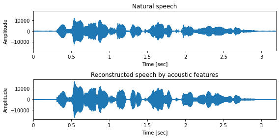
ax[0].set_title("Natural speech")
ax[1].set_title("Reconstructed speech by acoustic features")
librosa.display.waveplot(x.astype(np.float32), sr, ax=ax[0])
librosa.display.waveplot(y.astype(np.float32), sr, ax=ax[1])
for a in ax:
    a.set_xlabel("Time [sec]")
    a.set_ylabel("Amplitude")
plt.tight_layout()

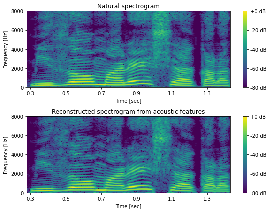
../_images/notebooks_ch05_DNNTTS_53_2.png

[31]:

n_fft =  1024
frame_shift = int(sr * 0.005)
X = librosa.stft(x.astype(np.float32), n_fft=n_fft, win_length=n_fft, hop_length=frame_shift, window="hann")
logX = librosa.amplitude_to_db(np.abs(X), ref=np.max)
Y = librosa.stft(y.astype(np.float32), n_fft=n_fft, win_length=n_fft, hop_length=frame_shift, window="hann")
log_Y = librosa.amplitude_to_db(np.abs(Y), ref=np.max)

fig, ax = plt.subplots(2, 1, figsize=(8, 6))
ax[0].set_title("Natural spectrogram")
ax[1].set_title("Reconstructed spectrogram from acoustic features")

mesh = librosa.display.specshow(logX, sr=sr, hop_length=hop_length, x_axis="time", y_axis="hz", cmap=cmap, ax=ax[0])
fig.colorbar(mesh, ax=ax[0], format="%+2.f dB")
mesh = librosa.display.specshow(log_Y, sr=sr, hop_length=hop_length, x_axis="time", y_axis="hz", cmap=cmap, ax=ax[1])
fig.colorbar(mesh, ax=ax[1], format="%+2.f dB")

for a in ax:
    a.set_xlabel("Time [sec]")
    a.set_ylabel("Frequency [Hz]")
    a.set_ylim(0, 8000)
    a.set_xlim(0.28, 1.43)
    a.set_xticks(np.arange(0.3, 1.4, 0.2))

plt.tight_layout()

# 図5-13
savefig("fig/dnntts_waveform_reconstruction")

../_images/notebooks_ch05_DNNTTS_54_0.png

第5章 深層学習に基づく統計的パラメトリック音声合成¶

準備¶

Python version¶

ttslearn のインストール¶

パッケージのインポート¶

描画周りの設定¶

5.3 フルコンテキストラベルとは？¶

モノフォンラベル¶

フルコンテキストラベル¶

5.4 言語特徴量の抽出¶

Open JTalk による言語特徴量の抽出¶

HTS 形式の質問ファイル¶

HTS 形式の質問ファイルの読み込み¶

フルコンテキストラベルからの数値表現への変換¶

言語特徴量をフレーム単位に展開¶

言語特徴量の可視化 (bonus)¶

5.5 音響特徴量の抽出¶

対数基本周波数¶

有声/無声フラグ¶

メルケプストラム¶

帯域非周期性指標¶

動的特徴量¶

音響特徴量の結合¶

5.6 音声波形の合成¶

第5章深層学習に基づく統計的パラメトリック音声合成¶